Circumference of an ellipse? Can't do it mate.

At the 2021 Sutton Trust summer school a student asked us for help with an integral she’d been struggling with:

\[\begin{equation} I = \int_0^a \frac{a^4 + (b^2 - a^2)x^2}{a^4 - a^2x^2}~{\mathrm{d}x}. \end{equation}\]

What followed was a dive down the rabbit hole of history, travelling from work of the mathematical greats to the depths of Google Group archives, all to answer one question: what’s the deal with the circumference of an ellipse?¹

What’s the problem?

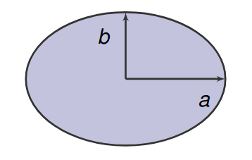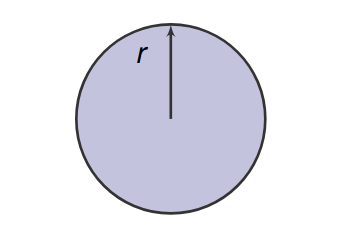
\(\text{Circle Area} = \pi r^2 \\ \text{Circumference} = 2\pi r\)	\(\text{Ellipse Area} = \pi ab \\ \text{Circumference} = \text{???}\)

We’re all taught in school that a circle with diameter \(2r\) has area \(\pi r^2\) and that its circumference is \(2\pi r\). You might have been taught that an ellipse with width \(2a\) and height \(2b\) has area \(\pi ab\), but what about its circumference? It turns out there’s no such ‘elementary’ equation for the circumference of an ellipse.

Why doesn’t it exist?

We remember from school that the arc length of a curve between \(x = x_1\) and \(x = x_2\), given in cartesian coordinates, is

\[s = \int_{x_1}^{x_2} \sqrt{1 + {\left( \frac{\mathrm{d}y}{\mathrm{d}x} \right)}^2}\mathrm{d}x.\]

If we first look at circle, when centred on zero² it has equation \(x^2 + y^2 = r^2\), so

\[\begin{align} y^2 = r^2 - x^2 &\Rightarrow y = \sqrt{r^2 - x^2} \\ &\Rightarrow \frac{\mathrm{d}y}{\mathrm{d}x} = -\frac{x}{\sqrt{r^2 - x^2}} \\ &\Rightarrow {\left( \frac{\mathrm{d}y}{\mathrm{d}x} \right)}^2 = \frac{x^2}{r^2 - x^2}. \end{align}\]

We can use the arc length equation to find the circumference, \(s\), of the circle. Using \(x_1 = 0\) and \(x_2 = r\) gives a quarter of the circumference, so

\[\begin{align*} s &= 4\int_0^r \sqrt{1 + \frac{x^2}{r^2 - x^2}}~{\mathrm{d}x} \\ &= 4\int_0^r \sqrt{\frac{r^2}{r^2 - x^2}}~{\mathrm{d}x} \\ &= 4\int_0^r \sqrt{\frac{1}{1 - {\left(\frac{x}{r}\right)}^2} }~{\mathrm{d}x} \\ &= 4{\left[ r\sin^{-1}\left(\frac{x}{r}\right)\right]}_0^r \\ &= 4r(\sin^{-1}1 - \sin^{-1}0) \\ &= 2\pi r. \end{align*}\]

That’s the circumference formula we all know and love! Ellipses are just squashed circles so logically the same should work for them right?

A standard ellipse with width \(2a\) and height \(2b\) has equation \(\frac{x^2}{a^2} + \frac{y^2}{b^2} = 1\). Another fact which will be useful later is that the eccentricity of an ellipse is given by \(k = \sqrt{1 - b^2/a^2}\). Working as before,

\[\begin{align} y^2 = b^2 - \frac{x^2 b^2}{a^2} &\Rightarrow y = \sqrt{b^2 - \frac{b^2}{a^2}x^2} \\ &\Rightarrow \frac{\mathrm{d}y}{\mathrm{d}x} = -\frac{b^2}{a^2}\cdot\frac{x}{\sqrt{b^2 - \frac{b^2}{a^2}x^2}} \\ &\Rightarrow {\left( \frac{\mathrm{d}y}{\mathrm{d}x} \right)}^2 = \frac{b^4}{a^4}\cdot\frac{x^2}{b^2 - \frac{b^2}{a^2}x^2}. \end{align}\]

Oh dear. For ellipses \(\frac{\mathrm{d}y}{\mathrm{d}x}\) is already more complicated than it was for circles, and that’s before we’ve even started integrating. Maybe there’ll be some cancellations though?

Using the equation for arc length as before with \(x_1 = 0\) and \(x_2 = a\) to find a quarter of the circumference gives

\[\begin{align} s &= 4\int_0^a \sqrt{1 + \frac{b^4}{a^4}\cdot\frac{x^2}{b^2 - \frac{b^2}{a^2}x^2} }{\mathrm{d}x} \\ &= 4\int_0^a \sqrt{1 + \frac{b^2 x^2}{a^4 - a^2x^2}}{\mathrm{d}x} \\ &= 4\int_0^{\frac{\pi}{2}} \sqrt{1 + \frac{(ab)^2\sin^2\theta}{a^4(1-\sin^2\theta)}} \cdot a\cos\theta~{\mathrm{d}\theta} \\ &= 4\int_0^{\frac{\pi}{2}} \sqrt{1 + \frac{b^2}{a^2}\frac{\sin^2\theta}{\cos^2\theta}} \cdot a\cos\theta~{\mathrm{d}\theta} \\ &= 4\int_0^{\frac{\pi}{2}} \sqrt{a^2\cos^2\theta + b^2\sin^2\theta}~{\mathrm{d}\theta} \\ &= 4\int_0^{\frac{\pi}{2}} \sqrt{a^2 + (b^2-a^2)\sin^2\theta}~{\mathrm{d}\theta} \\ &= 4a\int_0^{\frac{\pi}{2}} \sqrt{1 + \left(1 - \frac{b^2}{a^2} \right)\sin^2\theta}~{\mathrm{d}\theta} \\ &= 4a\int_0^{\frac{\pi}{2}} \sqrt{1 - k^2\sin^2\theta}~{\mathrm{d}\theta} \end{align}\]

at which point we stop and reconsider our life choices. This looks simple but just isn’t going anywhere.

This turns out to be what’s known as the complete elliptic integral of the second kind, a famously non-elementary integral. That is to say, it has no ‘nice’ solutions which means there isn’t an analogue to a circle’s \(2\pi r\) when looking at ellipses. To quote Gérard Michon:

There are simple formulas but they are not exact, and there are exact formulas but they are not simple.³

Showing why it’s non-elementary though goes beyond the scope of this post.

How can it be approximated?

Lets first look at the ‘simple’ formulas that aren’t exact. Over the years there have been many different attempts dreamt up for this, but if we’re wanting truly elementary formulas then we’ve a couple prominent options.

When doing his work on orbits Johannes Kepler (1609) used the geometric average, \(s \approx 2\pi\sqrt{ab},\) to approximate the circumference. It’s very poor with a worst case error of 100%, but it was over 400 years ago so what you gonna do.

About 170 years later, Leonhard Euler (1773) gave it a bash and figured out \(s\) can be bounded below by the arithmetic mean and above by the root mean squared,

\[2\pi\frac{a+b}{2} \leqslant s \leqslant 2\pi\sqrt{\frac{a^2 + b^2}{2}}.\]

More recently, Matt Parker (2020)⁴ debuted his lazy approximation,

\[s \approx \pi\left(\frac{6}{5}a + \frac{3}{4}b\right)~\text{where}~a\geqslant b,\]

which came from computational optimization: finding the numeral rational coefficients for an equation of that form which give the least error on average over a given range of \(a\).

It’s useful to see just how far off the truth these formulas are so we plot their deviation from the true circumference. Without loss of generality, we can vary the value of \(a\) while keeping \(b = 1\); we don’t care about orientation or scale.

Straight away we see that, with the possible exception of Lazy Parker, all these are pretty bad for anything except a very-round ellipse. Euler’s bounds are almost symmetrically bad and Kepler’s attempt shoots way off to the bottom, underestimating by almost 10% already by \(a = 2\).

The Lazy Parker approximation continues to beat these even at the extreme value of \(a = 20\), though by then it is underestimating by 3.43%. If we’re willing to add in some more bells and whistles though we can do better. These aren’t formulas you’d want to memorise but they will get you a good answer.

It wouldn’t be maths if Srinivasa Ramanujan (1914) didn’t have a finger in the pie, and he gave two pretty nice approximations:

1. \(s \approx \pi\left( 3(a+b) - \sqrt{(3a+b)(a+3b)} \right)\),
2. \(s \approx \pi(a+b)\left( 1 + \frac{3h}{10+\sqrt{4-3h}} \right) \text{ where } h = \frac{(a-b)^2}{(a+b)^2}\).⁵

The latter of these is astoundingly good as we’ll see in a moment. Parker also gave an coefficient-optimized solution mimicking the former,

\[\pi\left( \frac{53}{3}a + \frac{717}{36}b - \sqrt{269a^2 + 667ab + 371b^2} \right)~\text{where}~a\geqslant b\]

which has decent performance, though at the expense of complexity.

Far more recently, and coming from the unlikeliest of places, David Cantrell (2001) posted the following optimizable formula to a Google Group:

\[s \approx 4(a+b) - 2(4-\pi)\frac{ab}{H_p} \text{ where } H_p = {\left( \frac{a^p + b^p}{2} \right)}^{\frac{1}{p}}.\]

Here \(H_p\) is the Hölder mean. The value of \(p\) can be found through optimization or analysis, with \(p = (3\pi - 8)/(8-2\pi)\) working best for ‘round’ ellipses and \(p = \ln(2)/\ln(2 /(4-\pi))\) being optimal for ‘elongated’ ellipses. In practice, we can use \(p = 0.825\) which does just fine for everything.

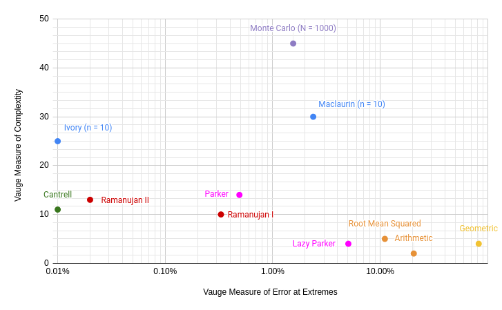
Though complicated approximations make for complicated graphs, all six of these approximations outperform all of our simple, rough approximations.

Ramanujan II is an incredible approximation and remains best right through to \(a = 20\), though Cantrell with \(p\) for elongated ellipses beats it soon after.

What if we look even further afield though, maybe at \(a = 75\)? At this point we might be tempted to stop and say

Who’s having an ellipse which is 75 times as wide as it is high? That’s just ridiculous! (Parker, 2020)

After all, even the orbit of Halley’s comet, famed for being highly elliptical, only has \(a = 3.93\) (an eccentricity of \(0.9671\)).

Well it turns out the most elliptical orbit we’ve discovered is of comet C/1965 S1-A Ikeya-Seki⁶. It has an eccentricity of \(0.999915\) giving \(a \approx 76.7 > 75\).⁷

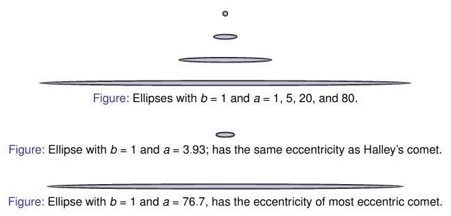
That’s a motivator to look further, up to \(a = 80\). There we see Ramanujan II has started to diverge more significantly from the truth and Cantrell’s approximation is winning out, particularly when

\[p = \frac{\ln(2)}{\ln\left( \frac{2}{4-\pi} \right)}\]

since it’s optimum for elongated ellipses.

All these approximations are pretty good and even the worst among them, Parker’s, stays within 0.5% error. If we want to find the actual circumference of an ellipse though we’ll have to look beyond these approximations. For that we now turn out attention to the exact formulas that are not simple.

How do we find it exactly?

There are three main power series used for ellipse circumferences: one from Colin Maclaurin (1742),

\[s = 2\pi a\sum_{m=0}^\infty \left( {\left( \frac{(2m)!}{m!m!} \right)}^2 \frac{k^{2m}}{16^m (1-2m)} \right)~\text{ where } k = \sqrt{1 - \frac{b^2}{a^2}},\]

one from Leonhard Euler (1776),

\[s = \pi\sqrt{2(a^2+b^2)}\sum_{m=0}^\infty \left( {\left(\frac{\delta}{16}\right)}^m \cdot \frac{(4m-3)!!}{(m!)^2} \right)~\text{ where } \delta = {\left( \frac{a^2-b^2}{a^2+b^2} \right)}^2,\]

and one from James Ivory (1796)⁸,

\[s = \pi(a+b)\sum_{m=0}^\infty \left( {\left( \frac{(2m)!}{m!m!} \right)}^2 \frac{h^m}{16^m {(1-2m)}^2} \right)~\text{ where } h = {\left(\frac{a-b}{a+b}\right)}^2.\]

While exact on paper these don’t converge in general. We can use them to approximate \(s\) by summing the first \(n\) terms of the power series. For example,

\[s \approx 2a\pi\sum_{m=0}^n \left( {\left( \frac{(2m)!}{m!m!} \right)}^2 \frac{k^{2m}}{16^m (1-2m)} \right)~\text{ where } k = \sqrt{1 - \frac{b^2}{a^2}}.\]

The amended plot below shows that summing Maclaurin’s series to \(n = 6\) is comparable to our rough approximations.

Similarly the plot below demonstrates that summing to \(n = 50\) is comparable to our higher accuracy approximations.

You might then think, okay, to find the exact circumference

Just use a power series to a high number of terms (Disney-Hogg, 2021)

but the practicalities turn out not to be so simple.

The convergence rate of Maclaurin’s series is slow. So slow in fact that the sum to \(n = 10\) terms already starts to diverge from the truth well before \(a = 20\) and is overestimating by 2.38% by the time \(a = 80\). Ivory’s series does fair far better, but for by \(a = 80\) for \(n = 10\) it’s also underestimating by 0.012%.

You might think, maybe we just need higher \(n\)? Well we can push both power series to \(n = 258\) terms⁹ and there is improvement. For Maclaurin it’s hardly the dizzying accuracy we might have hoped for, still being off by about 0.01% at \(a = 80\). That’s barely better than summing 10 terms Ivory, showing just how slow Maclaurin converges.

Meanwhile, even at \(a = 80\), \(n = 258\), Ivory is only producing an error of order \(10^{-11}\%\) which, let’s be fair, is pretty damn good. And that’s not even as far as we can take that series either! If we push it all the way to \(n = 507\) terms⁹, at \(a = 80\) we’re still within machine-epsilon error which is amazing.

In fact at \(n = 507\) we don’t start seeing numerical error until \(a \approx 140\), well beyond our known most elliptic orbits.

Carl Gauss (1812) & Eduard Kummer (1836)¹⁰ showed these three series could all be expressed in terms of the hypergeometric function:

\[\begin{align} \text{Maclaurin}: s &\approx 2\pi a\cdot {}_2F_1\left(-\frac{1}{2}, \frac{1}{2}, 1, k^2\right) \\ \text{Euler}: s &\approx \pi\cdot {}_2F_1\left(-\frac{1}{4}, \frac{1}{4}, 1, \delta \right) \\ \text{Ivory}: s &\approx \pi(a+b)\cdot {}_2F_1\left(-\frac{1}{2}, -\frac{1}{2}, 1, h \right) \end{align}\]

This coupled with the close proximity between the two findings means Ivory’s series is usually referred to as the Gauss-Kummer series.

R’s hypergeo package can evaluate this function, only returning an answer when the terms have converged within machine-epsilon error. Comparisons throughout this work use that function with blind faith that it’s more efficient and accurate than the best power series approximation we were able to use.

How could you do it with Monte Carlo?

The idea behind Monte Carlo integration is simple. To approximate

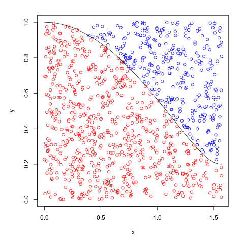
\[I = \int_0^\phi f(x){\mathrm{d}x}\]

we first plot \(f\) over \([0, \phi]\). Then we take \(N\) uniformly random points in a box \([0, \phi] \times [0,H]\) enclosing the plot, colouring them red if they fall below the integrand and blue if they fall above it. The integral approximation is then

\[I \approx (\phi-0) \times (H-0) \times \frac{\#\text{red}}{N}.\]

As the total number of random points increases the approximation converges toward the true value.

At first glance our initial integral

\[s = 4\int_0^a \sqrt{1 + \frac{b^2 x^2}{a^4 - a^2x^2}}{\mathrm{d}x}\]

isn’t lending itself to Monte Carlo integration. Not only do we have unknown \(a\) both in the integrand and in the limit, there’s also a lovely asymptote at \(x = a\). It’s not ideal for making a general tool.

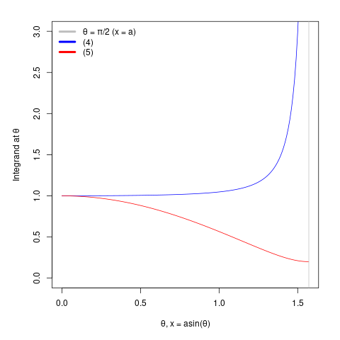
On the other hand, the transformation of that integral

\[s = 4a\int_0^{\frac{\pi}{2}} \sqrt{1 - k^2\sin^2\theta}~{\mathrm{d}\theta},\]

is far more inviting. The integrand plot can be enclosed by \([0,~\pi/2] \times [0,~1]\), making it a perfect candidate for doing Monte Carlo integration!

We coded up a simple function in R for doing this for arbitrary \(a\) and \(b\).

MonteCarlo = function(a, b, n=1e3, graph=FALSE) {
    # Given ellipse parameters 'a' and 'b' (where a >= b) and
    # sample count 'n' (default 1000) as inputs, this returns
    # an approximation of that ellipse's circumference using
    # Monte Carlo with n samples. If (optional) bool 'graph'
    # is TRUE (default FALSE) then a graph of the integrand
    # will be plotted.

    # calculate ellipse eccentricity
    k = sqrt(1-(b/a)^2);

    # upper integral limit, calculate 1/4 of ellipse then x4
    phi = pi/2;
    # integrand function, max of this is always 1
    f = function(x) { result = sqrt(1 - k^2 * sin(x)^2); }

    # generate random points in the box
    rand_x = runif(n, 0, phi);
    rand_y = runif(n, 0, 1);

    # true/false vector if each point was under graphs 
    under_integrand = rand_y < f(rand_x);
    # count the number of such points
    number_under_integrand = sum(under_integrand);

    # monte carlo estimation of the area under the graph
    area = phi * 1 * (number_under_integrand/n)

    # optional, graphs integrand and the approximation samples
    if (graph) {
        png("Figs/mc-graph.png")
        par(mar=c(5,5,2,2)+0.1) # remove title space
        # trace out the integrand
        x = seq(0, phi, 0.01);
        y = f(x);
        plot(x, y, type='l', xlim=c(0, phi), ylim=c(0,max(y)))
        # obligatory red/blue MC graph points
        points(rand_x[under_integrand],
               rand_y[under_integrand],
               col="red")
        points(rand_x[!(under_integrand)],
               rand_y[!(under_integrand)],
               col="blue")
        dev.off()
    }

    # final result is 4a times the integral
    return(4*a*area)
}

We’re not the first to apply Monte Carlo to this problem; Gary Gipson (1982) explored the idea more generally as part of his PhD thesis.¹¹

To give a specific example, if we have \(a = 5\), \(b = 1\), our true circumference is \(21.01004\). Carrying out Monte Carlo integration might look as below.

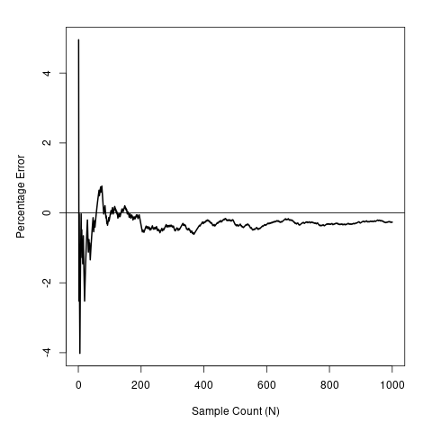Example graph output from the MonteCarlo function.	Example convergence plot as more samples are added.

In particular, the graph on the left approximates the ellipse’s circumference as

\[s \approx 4a \times \left(\frac{\pi}{2}\times1\right) \times \frac{684}{684 + 316} = 21.48849,\]

meaning there’s about 2% error. To see how this compares in absolute value terms, the table below has all our approximations all side by side for varying \(a\).

Method	\(a = 1\)	\(a = 5\)	\(a = 20\)	\(a = 80\)
Arithmetic Average	6.283185	18.84956	65.97345	254.4690
Geometric Average	6.283185	14.04963	28.09926	56.1985
Euler Average	6.283185	22.65435	88.96866	355.4584
Ramanujan I	6.283185	21.00560	80.24683	319.0854
Ramanujan II	6.283185	21.01003	80.38430	320.0634
Parker	6.282953	21.00714	80.17898	318.5687
Lazy Parker	6.126106	21.20575	77.75442	303.9491
Cantrell, \(p = 0.825\)	6.283185	21.00887	80.39483	320.1485
Maclaurin, \(n = 10\)	6.283185	21.18883	82.11027	327.7535
Ivory, \(n = 10\)	6.283185	21.01004	80.38718	320.0904
Monte Carlo, \(N = 10^3\)	6.283185	21.55133	80.42477	315.1646
Truth	6.283185	21.01004	80.38851	320.1317

We can see that Monte Carlo isn’t terrible, but it’s also not as good as some of even our more basic approximations like Parker. That begs the question…

Why use Monte Carlo to approximate circumference?

Given Monte Carlo isn’t more efficient, more accurate, or simpler to state than any of the other approximations given here there’s not a clear reason to use it beyond academic curiosity. A better question though might be…

Why use ellipses to demonstrate Monte Carlo?

Monte Carlo approximations aren’t difficult to understand; I’ve a memory of being taught the basics around Y8 (12 years old). We were given a coin to toss 100 times, recording the results and working out the approximate probability of heads by dividing the number of times it happened by 100. It’s not a very exciting demonstration, but it works.

That’s for showing it to a younger audience though, what about when you’re showing it to undergrads? The go-to examples are integration or calculating \(\pi\).

As we did for our elliptic integral, given \(p(x) = a_n x^n + a_{n-1}x^{n-1} + \cdots + a_0\) we can approximate \(\int_{x_1}^{x_2} p(x){\mathrm{d}x}\) by generating \(N\) uniform random points in a box bounding \(p\) between \(x_1\) and \(x_2\), counting the number of that fall below \(p\) and dividing that by \(N\). While the idea is still simple, it’s not exactly interesting and feels pretty redundant; polynomial integration can be done exactly and is borderline trivial for most undergrads. Even if \(p\) were to be more complicated, students will be painfully aware there are better approximation methods.

Approximating \(\pi\) has other problems. It’s still integral approximation at heart so it’s not complicated, but it has the aura of a pointless exercise. It does have the advantage of being a well known constant and seeing the approximation converge is a neat demonstration, but how Monte Carlo is being used here is very specific to \(\pi\) and not widely applicable.

Putting aside that it’s not necessarily the best tool for the job, there are some benefits to using ellipse circumference in a Monte Carlo demonstration:

• Unlike approximating \(\pi\), the Monte Carlo integration method used is more widely applicable outside the given context;
• At the same time, unlike \(p(x)\), we don’t have an elementary integral so using an approximation method to find an answer is practical;
• That we don’t have an elementary equation for an ellipse’s circumference is interesting and not a fact all undergrads will have come across;
• The math needed to understand what’s going on is perfectly suited for early undergrads (arc length, integration by substitution, etc), while not being out of reach for enthusiastic sixth-formers.

A downside to bare in mind that it prompts the question, ‘why is this integral non-elementary?’ to which there’s no easy answer; get your references to take higher year integrability courses at the ready!

That aside though, Monte Carlo Elliptic Integrals is a neat tool being applied to an cool problem in a way that’s both interesting and understandable. It’s a good motivator for why Monte Carlo methods might be useful in a practical setting while not presenting an application beyond the understanding of a novice mathematician.

---

Footnotes & References

1. This post mirrors a talk I gave called Monte Carlo Elliptic Integrals at the Maxwell Institute Graduate School’s PG Colloquium in October 2021. Thanks to Andrew Beckett for working through the original integrations, Linden Disney-Hogg for his insights into integrability, Chris Eilbeck for pointing me toward further research, and of course to Callie for introducing me to the problem. ↩

2. Throughout we can center circles and ellipses on zero without loss of generality; relative position has no baring on circumference. Similarly, when working with ellipses we don’t have to concern ourselves with how they’re oriented. ↩

3. G. P. Michon, Final Answers, ch. Perimeter of an Ellipse. Numerica, 2004, most recently updated 2020. A fabulous literature review without which this post wouldn’t have been possible. ↩

4. M. Parker, Why is there no equation for the perimeter of an ellipse!?, YouTube, September 2020. Another great review of the topic and the source of Parker’s computationally optimized simple formulas. ↩

5. \(h\) crops up a lot but, according to Michon, it’s an unnamed quantity. ↩

6. Jet Propulsion Laboratory, C/1965 S1-A (Ikeya-Seki), Small-Body Database, 2008. The source of the values in working out the orbit with the highest known eccentricity. ↩

7. This is so perfectly close to Parker’s ‘ridiculous’ value for \(a\) that I don’t know if it’s an intentional easter egg or just coincidence. ↩

8. Despite the name, the Gauss-Kummer series first appeared in a memoir of Scottish mathematician and University of Edinburgh alumni, Sir James Ivory: A new series for the rectification of the ellipse, Transactions of the Royal Society of Edinburgh, vol. 4, no. II, pp. 177–190, 1796. ↩

9. When coding these approximations we used R; it made sense in the Monte Carlo context and it was what we’d for other aspects of the summer school. As a language though, it’s very limited in how it handles large numbers. In particular, using factorial to compute \(n!\) for \(n > 170\) just returns \(\infty\), a problem for Maclaurin since it includes a \((2n)!\) term. At face value we’re thus limited to summing the first \(n = 85\) terms, a problem given its slow convergence rate. It’s possible to improve that limit to \(n = 258\) using choose or lfactorial, though it’s arguable how useful that is given it’s still producing an error of \(10^{-3}\%\) compared to Ivory’s \(10^{-11}\%\). Ivory has an upper limit of \(n = 507\) before R gets angry for similar reasons, and that’s sufficient to handle to \(a\) up to 140. ↩ ↩²

10. P. Abbot, On the perimeter of an ellipse, The Mathematica Journal, vol. 11, no. 2, 2011. Originally presented at the International Mathematica Symposium 2006. ↩

11. G. Gipson, The Coupling of Monte Carlo Integration with the Boundary Integral Equation Technique to Solve Poisson Type Equations, PhD Thesis, Louisiana State University, 1982. ↩